Data Analysis with R I: Normalization and Frequency Distribution
What this document does
- normalizes frequencies of a given data set relative to a subcorpus or other relevant token size (e.g. number of verbs in subcorpus)
- produces a frequency distribution graph of the normalized data
- produces a sortable data table of the normalized data
The document uses two R-functions from the R-script func_dataana_normfreq.R - norm.data - plot.bar
The functions facilitate normalization and plotting making the R-Markdown more readable and easier to modify.
Getting started
- download
- the zip-file including the R Markdown file (.Rmd), an R-script (.R) with functions as well as the sample data
- unpack the zip-file in the course directory
- open the R Markdown file (
Data_analysis_norm-and-freq.Rmd) in RStudio - if you klick on
Knitit will generate a HTML document including both text content and the output of the embedded R code chunks - you can delete and/or change any text (white background) without affecting the functionality of the document
Input data
The document requires two different data sets.
- data set of phenomena
- data set with subcorpus frequencies (the subcorpus frequencies are not needed if you can calculate the relative token size from the data set)
Initially the file runs with the sample data provided:
- sample data set: Full verbs and their parts-of-speech across registers and corpora (BROWN, FROWN, BLOB, FLOB, LOB) in the Brown family corpora
- sample data set with subcorpus frequencies (register and corpora)
See Creating the sample data for information on how to create the sample data provided.
You may also use the document with your own data. In this case you simply have to adjust the parameters below.
- See Download query results in a TAB-deliminated format for more information on data sets and how to extract them using CQPweb.
- See Manipulating Data Sets for information on how to modify an existing data set (adding columns, etc.)
Parameter settings: you need to adopt the variables in this chunk to process your own data or to change the features for the analysis.
# Parameter settings: ADOPT this variables in this chunk to process your own data
# data set file with column names
datafile <- "data/distr_vfull_lemma-pos-reg-sc_brownfam-meta.txt"
# data set with token sizes with column names
csizefile <- "data/brown_family_csizes-meta.txt"
Analysis
The first thing we have to do is load the data sets.
As you can see, the r-chunk uses the parameters we set above to load the data sets dat and d.csize.
# load the data set file
dat <- read.table(datafile, header=T, fill=T, sep="\t", row.names=NULL, quote="")
# load the data set with token sizes
d.csize <- read.table(csizefile, header=T, fill=T, sep="\t", row.names=NULL, quote="")
The data set dat is a multivariate data set including a lot of different features, e.g. the verb lemma and the part-of-speach as well as register, language variety, and year.
We can choose which features we want to investigate more closely using the paramter variables feat1 and feat2.
In this tutorial feat1 refers to the linguistic phenomenon, while feat2 refers the subcorpus.
We can change the features any time to plot new things.
General process
- setting parameters (
feat1andfeat2) - normalize the data
- plot the data
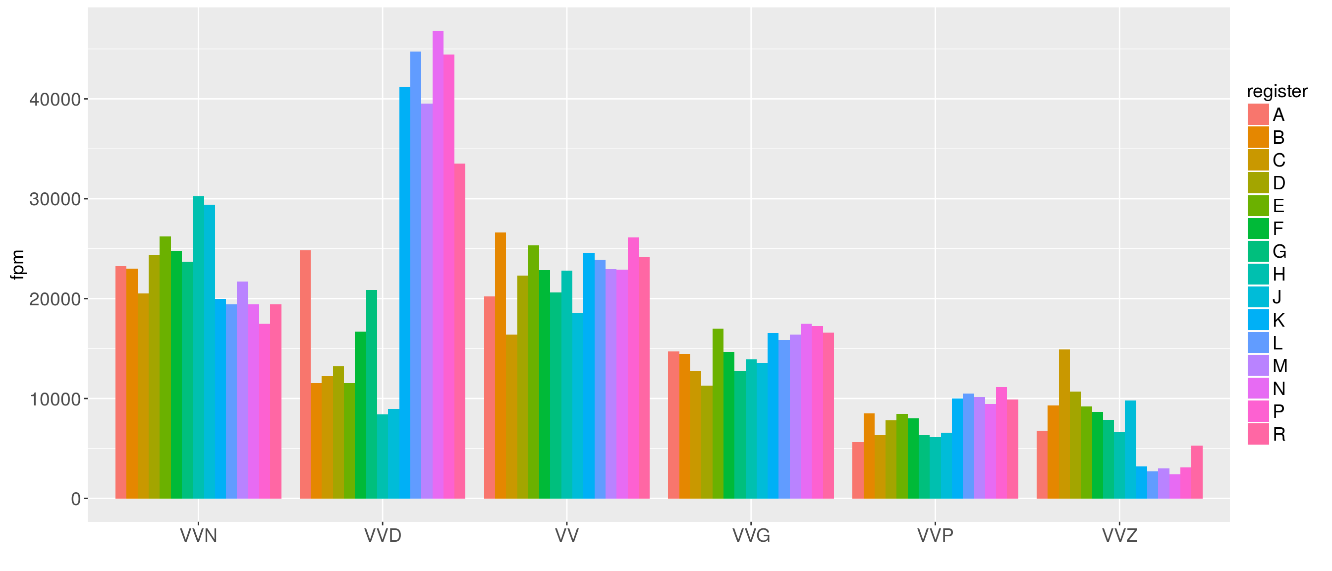
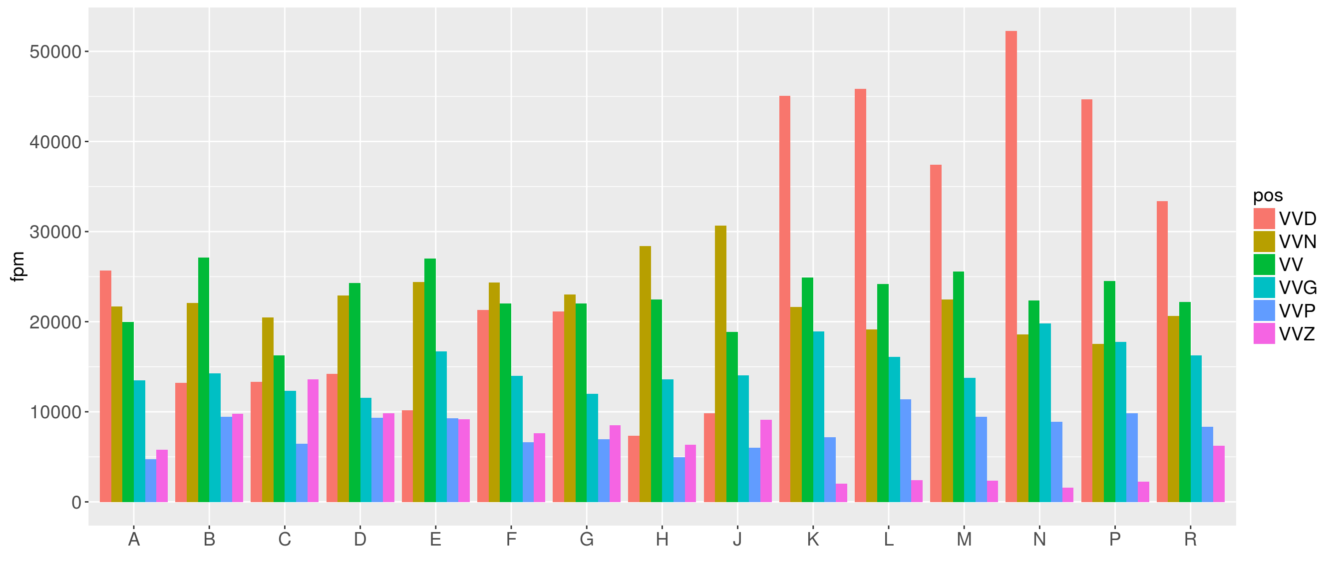
Our first plot show the distribution of parts-of-speech across registers.
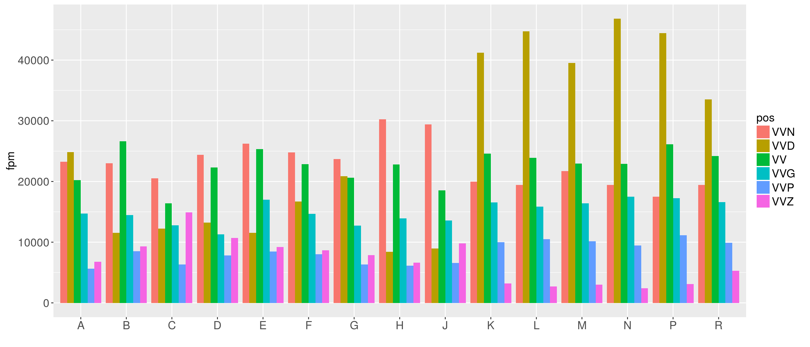
We can also easily turn the diagram:
You can also make the plot interactive
Changing parameters
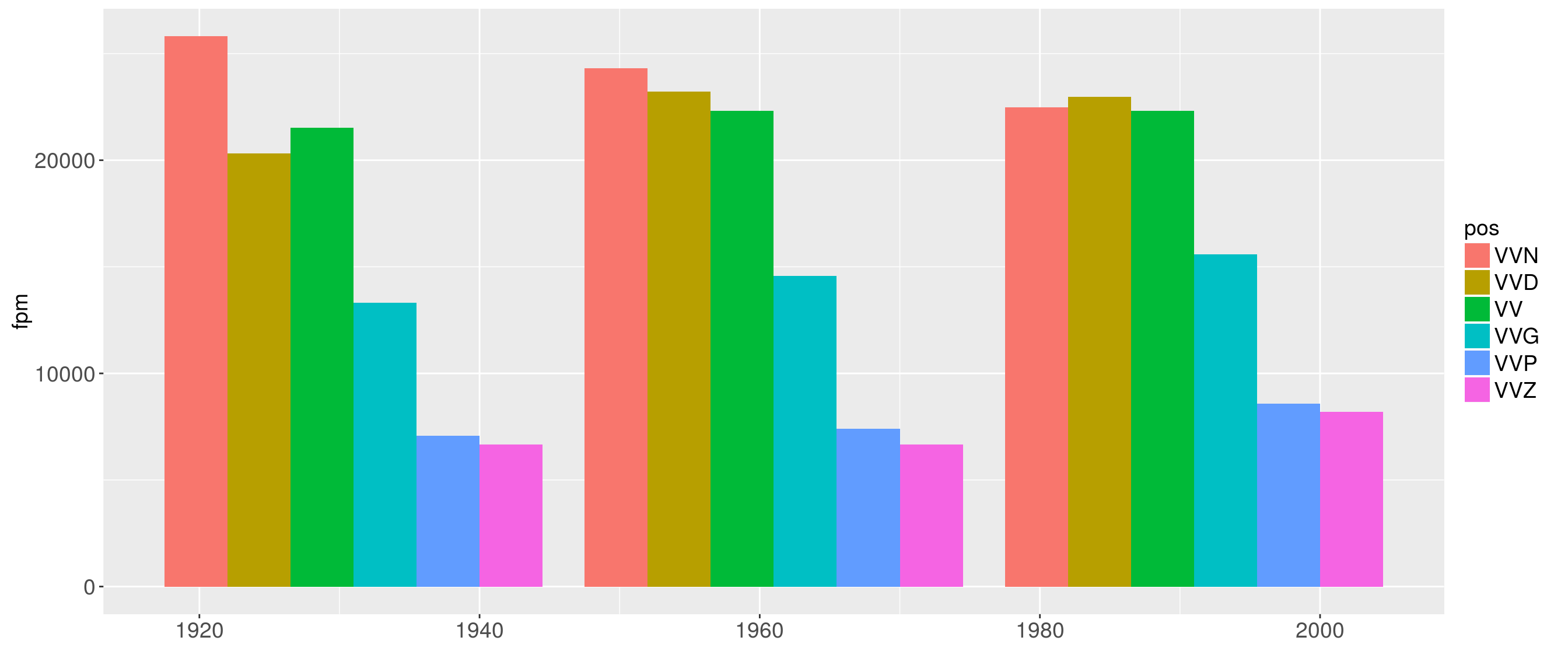
Now we want to have a look at the distribution of parts-of-speech across time (year)
Plotting subsets
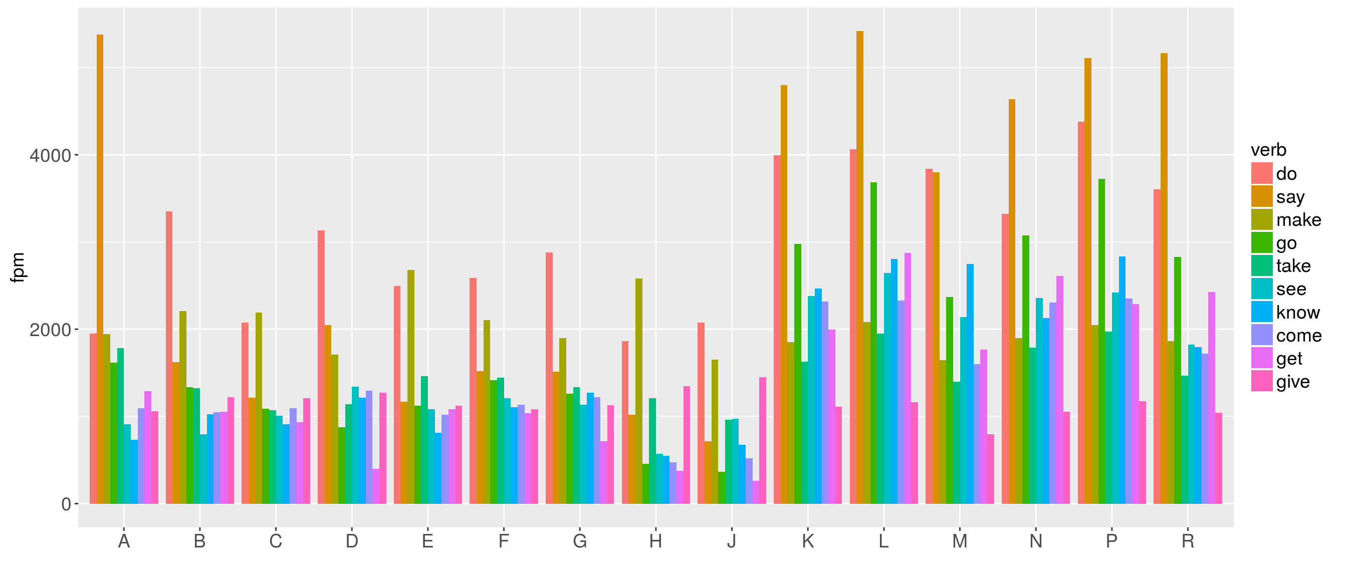
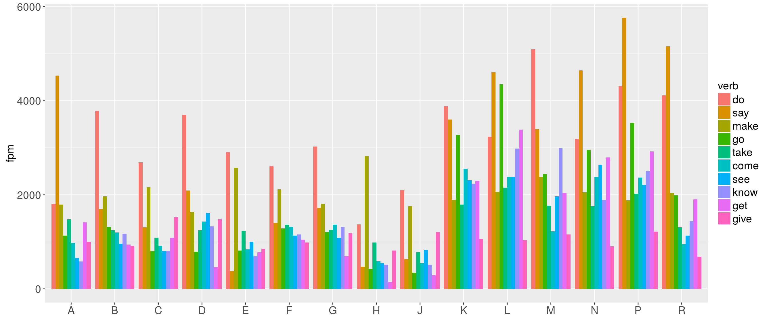
Now we want to have a look at the distribution of verb lemmas. However, we want to plot the 10 most frequent verb lemmas only.
Exercises
Exercise 1
What if we want to see the distribution of the parts-of-speech across registers in different subcorpora, e.g. the BROWN corpus.
Then we have to
- build subsets including only the BROWN corpus data
- normalize the data using the subsets
- plot the subsets
- Plot the same parameters for the BLOB corpus and compare.
- Compare the results.
- Make notes of your observations.
Exercise 2
The following plots the 10 most frequent verb lemmas in the BROWN corpus.
Plot the same for the BLOB corpus and compare. Make notes of your observations.
Exercise 3
Plot the following
- distribution of the 10 most frequent verb lemmas across language varieties
- distribution of parts-of-speech across language varienties
- make notes about your observations